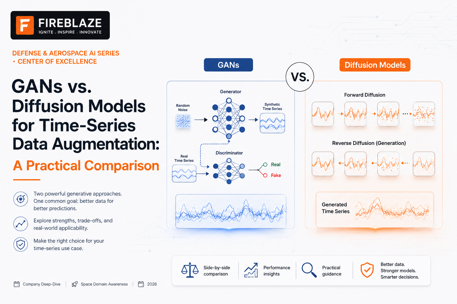
GANs vs. Diffusion Models for Time-Series Data Augmentation: A Practical Comparison

Part of our GenAI-Augmented Predictive Maintenance for Jet Engines series — the architectural deep dive our rare-failure-mode primer promised, written for the reader who's about actually to pick one and implement it.

1. Hook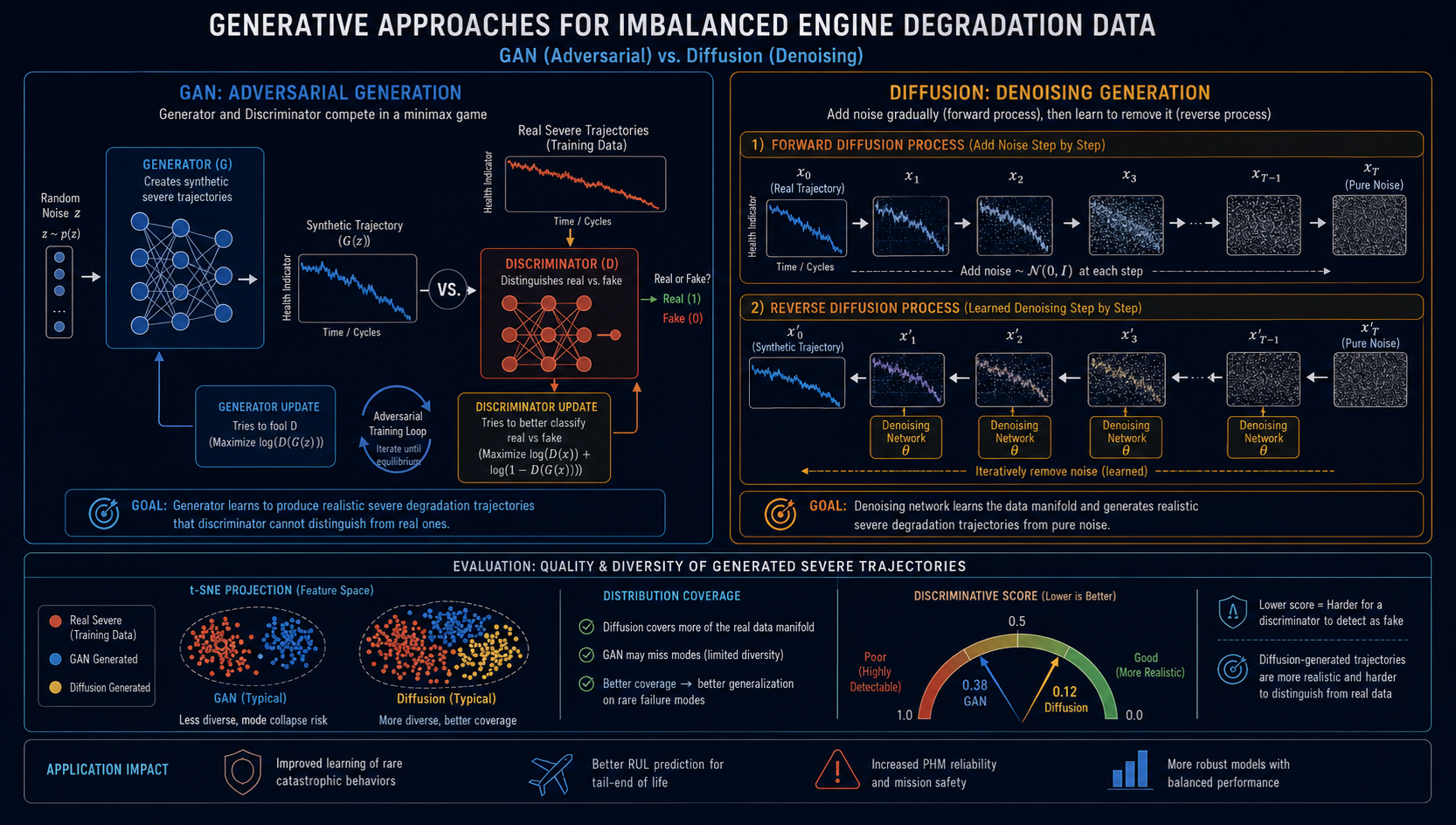

Every published comparison of GANs and diffusion models eventually says some version of "diffusion models are more stable but more expensive" and leaves it there — which is true, but it's the least useful part of the answer for someone actually choosing between them for a specific time-series augmentation task. The real decision hinges on details most surveys skip entirely: how you'll evaluate whether the synthetic data is any good, how long your sequences are, how much compute and wall-clock time you actually have, and which specific architecture within each family has been validated on data that looks like yours. This piece is the practical version of that decision.

2. Core Explanation

2.1 The Same Two Ideas, Restated Precisely

Both architectures were introduced in our companion piece on rare failure modes, but a practical comparison needs a more precise restatement of the actual mechanics, because the implementation differences that matter downstream all trace back to these mechanics.

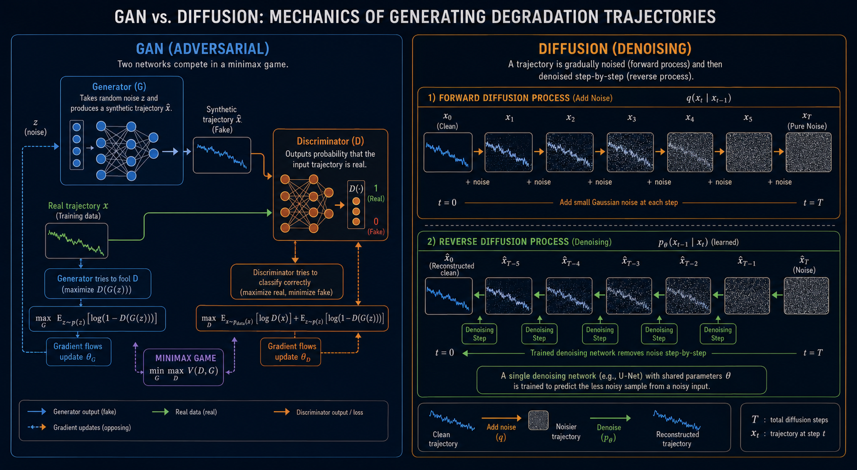
A Generative Adversarial Network (GAN) frames generation as a minimax two-player game: a generator network G maps random noise to synthetic samples, and a discriminator network D is trained simultaneously to classify samples as real or synthetic. The generator's objective is to maximize the discriminator's error rate; the discriminator's objective is to minimize it. Training alternates between updating each network against the other, and convergence — in principle — occurs when the generator produces samples the discriminator can no longer distinguish from real data at better than chance.

A diffusion model frames generation completely differently, as a Markov chain denoising problem. A forward process incrementally adds Gaussian noise to real training data across many steps (often in the hundreds to low thousands) until the data is indistinguishable from pure noise. A single neural network is then trained to reverse this — given a noisy sample and a timestep, predict the noise that was added, so that noise can be progressively subtracted step by step, starting from pure random noise, until a realistic sample emerges. Critically, there is no adversary in this setup: the network's training signal is a direct, well-behaved denoising loss, not the output of a second network trying to defeat it.

This structural difference — a fragile two-network equilibrium versus a single network solving a well-posed denoising regression — is the root cause of essentially every practical tradeoff discussed in the rest of this piece, so it's worth keeping in mind as the throughline underneath every comparison below.

2.2 How the Field Actually Measures "Is This Synthetic Data Any Good"

Before comparing architectures, it's essential to understand the evaluation protocol the time-series generation literature has converged on, because without it, "GAN vs. diffusion" comparisons are just vibes. Since the original TimeGAN paper established the convention, three metrics have become close to a de facto standard, appearing consistently across nearly every subsequent time-series generation paper — TimeVAE, ChronoGAN, DLGAN, SeriesGAN, Diffusion-TS, and TIMED among them:

Discriminative score — train a classifier (typically a 2-layer GRU or LSTM) to distinguish real sequences from synthetic ones on a held-out set, then report the classifier's accuracy minus 0.5. A score near 0 means the classifier essentially can't tell real from synthetic — the ideal outcome. A score near 0.5 means the synthetic data is trivially distinguishable from real data, i.e., a poor generator.
Predictive score — train a sequence model (again, typically a small GRU or LSTM) purely on the synthetic data to forecast next-step values, then evaluate that model's mean absolute error on real held-out data. This directly tests whether the synthetic data preserved the temporal dependency structure well enough for a downstream model trained on it to generalize to real sequences — arguably the single most operationally relevant of the three metrics for an augmentation use case.
Distributional visualization (t-SNE / PCA) — project both real and synthetic sequences into two dimensions and visually inspect how much their distributions overlap. This is qualitative rather than a single number, but multiple papers note it catches failure modes the two quantitative scores can miss — specifically, a generator that has learned only part of the real data's distribution well (producing high-quality samples for a subset of the pattern space while badly under-covering the rest) can still post a deceptively good discriminative or predictive score.

A newer complementary metric, Context-FID (Context-Frechet Inception Distance), adapts the Frechet Inception Distance concept from image generation to time series by replacing the image-domain Inception network with a time-series representation-learning model (TS2Vec), producing a single distributional-distance number where lower indicates the synthetic sequences sit closer to the real data distribution in a learned representation space.

The practical point worth internalizing here: any credible comparison between a GAN and a diffusion model for your specific use case should report at minimum the discriminative and predictive scores on your actual data, not just training-loss curves or a handful of visually inspected example plots — because as the mode-coverage caveat above illustrates, a model can look impressive on hand-picked examples while systematically failing on a meaningful portion of the real distribution's diversity.

Metric	What It Measures	Good Score	What It Catches That Others Miss
Discriminative score	How distinguishable synthetic data is from real data	Close to 0	Overall realism at the sequence level
Predictive score	Whether temporal dependencies transfer to real data	Low MAE	Whether the synthetic data is actually useful, not just realistic-looking
t-SNE / PCA overlap	Visual distributional coverage	High overlap, no isolated clusters	Partial mode coverage — good on some patterns, bad on others
Context-FID	Distributional distance in a learned representation space	Low	A single-number distributional summary, complementary to discriminative/predictive scores

2.3 The GAN Family: What's Actually Been Built for Time Series

Plain, unmodified GAN architectures (designed originally for images) transfer poorly to time series, because they have no inherent mechanism for enforcing temporal coherence across a sequence. This gap has produced a well-developed lineage of purpose-built variants worth knowing by name, since "GAN" alone is not a specific enough answer to "which architecture should I use":

TimeGAN (Yoon et al., 2019) is the foundational architecture most later work benchmarks against. It combines an adversarial network with a supervised autoregressive component and a jointly-trained autoencoder, embedding sequences into a lower-dimensional latent space before applying adversarial training there rather than on raw sequences directly — a design specifically meant to help the generator learn stepwise temporal dynamics rather than just marginal per-timestep statistics.
RCGAN / TTS-GAN / TTS-CGAN extend the conditional-GAN concept (where generation can be conditioned on a class label or attribute) into the time-series and transformer domains respectively, useful specifically when you need to generate synthetic sequences of a particular labeled failure type rather than generic synthetic data — directly relevant to the failure-type-aware augmentation approach discussed in our rare-failure-modes piece.
DLGAN and ChronoGAN are more recent architectures that report measurable improvements over TimeGAN on standard benchmark datasets — DLGAN separates feature-matching from sequence-reconstruction into a two-stage adversarial framework, while ChronoGAN reports substantially lower discriminative scores than TimeGAN across several benchmark datasets in its published comparisons.
DoppelGANger, developed originally for networked time-series data sharing, is notable less for its architecture and more for a practical engineering result: a PyTorch reimplementation by Gretel reported roughly a 40x runtime speedup over the original TensorFlow implementation on a real synthesis task — a useful reminder that implementation and framework choice, not just architecture choice, materially affects the practical cost comparison between approaches.
WGAN-GP (Wasserstein GAN with Gradient Penalty) isn't time-series-specific but is frequently layered underneath time-series GAN variants specifically to address the training-instability problem, by replacing the original GAN's divergence measure with the Wasserstein distance — a change that directly targets and reduces (though does not eliminate) mode collapse risk.

The consistent theme across this lineage: each successive architecture is, in large part, a response to a specific weakness observed in its predecessor, usually either training instability, insufficient temporal coherence, or incomplete mode coverage — which tells you something important about the family as a whole: it has needed continuous architectural intervention to compensate for weaknesses that are fairly fundamental to the adversarial training paradigm itself, rather than incidental bugs.

2.4 The Diffusion Family: A Newer but Rapidly Maturing Lineage

Diffusion-based time-series generation is younger than the GAN lineage above, but has moved fast, and several architectures are now directly benchmarked against the TimeGAN-era GAN baselines using the same discriminative/predictive score protocol described in Section 2.2:

Diffusion-TS frames itself explicitly as an interpretable diffusion model for general time-series generation, decomposing generated sequences into trend and seasonal components — a design choice aimed at making the generation process more transparent and controllable than a typical black-box denoising network, which matters for a use case where you may specifically want to control or verify what kind of degradation trend is being synthesized.
TransFusion combines diffusion with transformer architecture specifically to extend the usable sequence length for time-series generation, reporting successful generation at a sequence length of 384 — notably longer than the sub-100-length sequences most earlier GAN-based approaches were evaluated on, directly relevant to jet-engine degradation trajectories that can span hundreds of cycles.
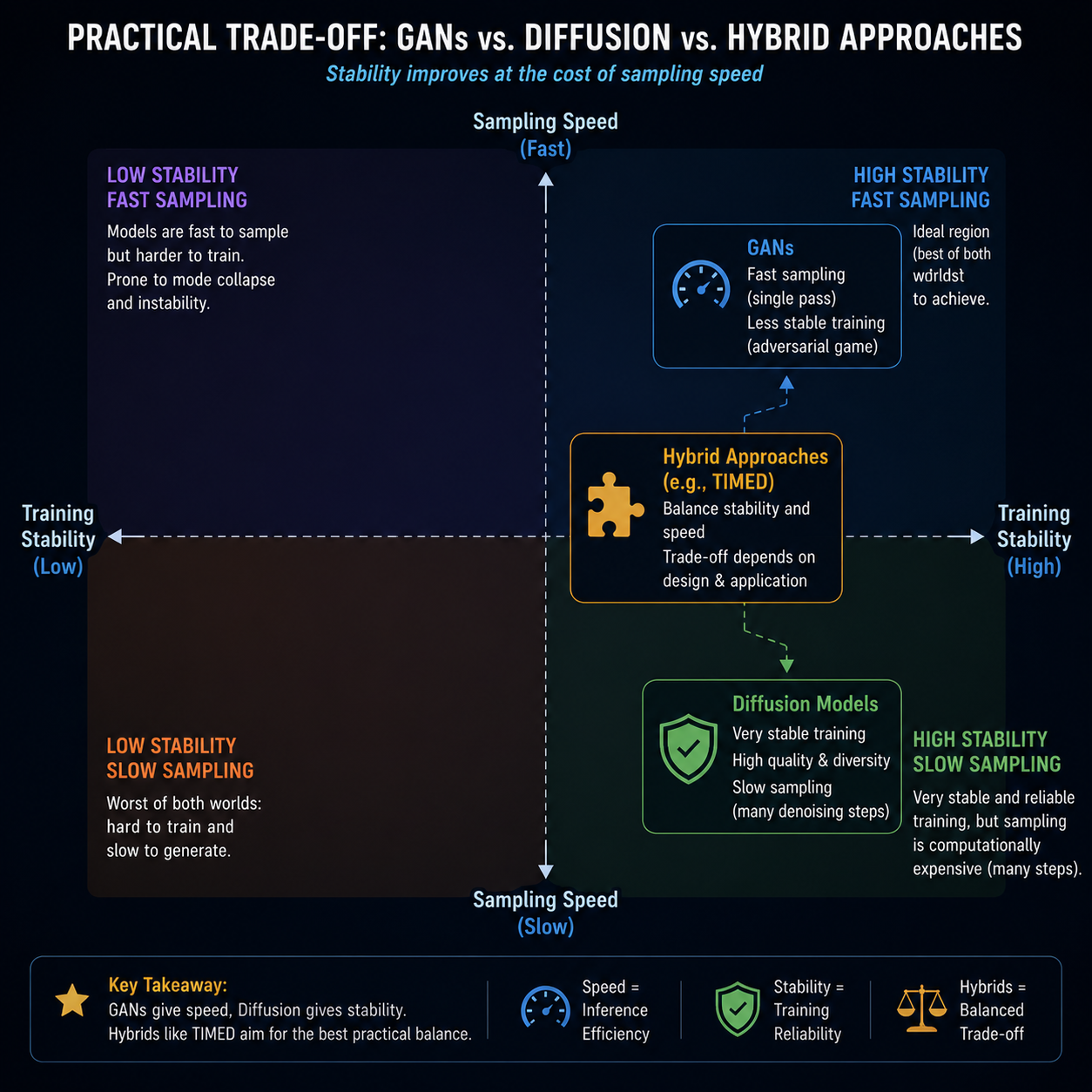
TIMED takes a hybrid approach worth noting specifically because it complicates the "GAN vs. diffusion" framing as a strict either/or: it applies adversarial and autoregressive refinement on top of a diffusion-based backbone, explicitly trying to combine diffusion's training stability with adversarial training's sharpening effect on sample fidelity — suggesting the field's frontier may be converging toward hybrids rather than a clean architectural fork.
DS-Diffusion focuses specifically on style-guided generation, incorporating external conditioning (extracted via transformer or GRU components) to control the "style" or pattern characteristics of generated sequences — directly relevant to the failure-type-conditioned generation use case flagged in Section 2.3 above for the GAN family, showing this capability isn't GAN-exclusive.

Across this lineage, several published architectural comparisons converge on the same qualitative finding already introduced in our companion rare-failure-modes piece: diffusion models exhibit smoother, more stable training loss curves with fewer of the oscillating generator/discriminator dynamics that characterize adversarial training, and better mode coverage — meaning less risk of the generator collapsing onto reproducing a narrow subset of the training distribution. The tradeoff, also consistent across sources, is compute: one controlled architectural comparison study found diffusion models required roughly 400 seconds per training iteration versus roughly 40 seconds per epoch for GANs in the same experimental setup — an order-of-magnitude difference that compounds significantly across a full training run and across any hyperparameter search.

2.5 A Direct, Practical Comparison Table

Bringing the two lineages together against the dimensions that actually drive a real implementation decision:

Dimension	GAN Family	Diffusion Family
Training objective	Adversarial minimax game between generator and discriminator	Direct denoising regression loss, no adversary
Training stability	Prone to oscillation and mode collapse; often needs stabilization tricks (gradient penalty, spectral normalization)	Generally smooth, stable convergence out of the box
Mode coverage	Weaker — the classic failure mode is exactly the diversity loss most damaging for rare-case augmentation	Stronger — better coverage of the true data distribution in most published comparisons
Training compute cost	Lower per-iteration cost; faster to iterate on architecture/hyperparameter choices	Substantially higher — roughly an order of magnitude slower per iteration in controlled comparisons
Sampling (inference) cost	Fast — typically a single forward pass through the generator	Slow — requires the full iterative denoising chain (though accelerated samplers reduce this gap)
Maturity for long sequences	Well-established at short-to-moderate lengths (sub-100 to ~200 steps); longer sequences historically harder	Actively improving — TransFusion demonstrates successful generation at 384-step sequences
Controllability / conditioning	Well-supported via conditional variants (RCGAN, TTS-CGAN)	Increasingly supported via style/condition-guided variants (DS-Diffusion)
Known failure signature	Mode collapse — synthetic diversity that's actually near-duplication	Smoothing bias — may under-represent sharp, volatile signal characteristics
Best-fit scenario	Fast iteration cycles, ample compute-time constraints, shorter sequences, well-understood conditioning needs	Longer sequences, priority on distributional diversity and rare-pattern coverage, more tolerance for training/sampling cost

For the specific case of rare-failure-mode trajectory augmentation in jet-engine RUL data — the direct throughline from our companion piece — the mode-coverage argument matters disproportionately, because the entire point of the exercise is capturing diversity in an already-sparse minority class; a GAN that mode-collapses onto near-duplicates of the two or three real examples it has to work from produces exactly the failure this whole exercise exists to avoid. This tilts the practical recommendation, all else equal, toward diffusion-based or hybrid (TIMED-style) approaches specifically for this use case, with the caveat that the compute cost tradeoff is real and should be weighed against available project resources rather than treated as automatically worth paying.

2.6 The Practical Toolkit: What You'd Actually Reach For

Beyond the research architectures named above, several open-source frameworks package these techniques into usable libraries, and knowing the landscape matters for anyone actually starting an implementation rather than a literature review:

TSGM (Time Series Generative Modeling), presented at NeurIPS 2024, is an open-source framework specifically for synthetic time-series generation and evaluation, implementing multiple generator families (including GAN-based and VAE-based approaches) alongside built-in evaluation metrics for consistency, privacy, and downstream performance, and providing access to over 140 benchmark datasets — a genuinely useful starting point for anyone wanting to benchmark multiple architectures without reimplementing each from its original paper.
ydata-synthetic (recently renamed fg-data-synthetic) provides a lower-code interface for generating both synthetic tabular and time-series data using several generative model families, including a Streamlit-based UI for interactive use.
SDV (Synthetic Data Vault) is one of the earliest and most established open-source synthetic data projects, covering tabular, relational, and time-series data generation, though its time-series-specific generative capabilities are less specialized than purpose-built time-series frameworks like TSGM.
gretel-synthetics, an open-source library from Gretel, includes a PyTorch reimplementation of DoppelGANger, notable for the significant runtime improvement over the original implementation mentioned in Section 2.3.

For a project already working in a Python/PyTorch or TensorFlow environment on C-MAPSS-style trajectory data, the realistic starting point is rarely "implement TimeGAN or Diffusion-TS from the original paper" — it's evaluating whether TSGM's built-in generator zoo already covers a close enough architectural match, and reaching for a from-scratch or heavily customized implementation only once that off-the-shelf option has been evaluated and found insufficient for the specific trajectory-shape and conditioning requirements at hand.

2.7 A Decision Framework, Not Just a Recommendation

Given everything above, the honest answer to "which should I use" is genuinely conditional, and it's more useful to lay out the actual decision logic than to declare a universal winner:

If your sequences are short (well under 100 steps) and you need to iterate quickly through many architecture and hyperparameter variations, the lower per-iteration cost of a GAN-based approach (starting from TimeGAN or a conditional variant like TTS-CGAN if you need failure-type conditioning) is likely to get you to a usable result faster, provided you budget real engineering time for stabilizing training and actively monitoring for mode collapse via the discriminative score and t-SNE visualization from Section 2.2 — not just training-loss curves, which can look fine even as mode collapse is occurring.
If your sequences are long (multiple hundreds of steps, closer to a full C-MAPSS engine trajectory) and distributional diversity on a sparse minority class is the primary goal, a diffusion-based approach (Diffusion-TS or TransFusion as a starting architecture) is the better-supported choice in the current literature, provided your compute budget can absorb the roughly order-of-magnitude higher training cost documented in Section 2.4.
If you need explicit conditioning on failure type (echoing the multi-generator, failure-type-aware architecture discussed in our rare-failure-modes piece), both families now support this — RCGAN/TTS-CGAN on the GAN side, DS-Diffusion-style conditioning on the diffusion side — so this requirement alone shouldn't be the deciding factor between families.
Regardless of which family you choose, budget real evaluation effort for Section 2.2's protocol — discriminative score, predictive score, and distributional visualization, at minimum — rather than declaring success based on visual inspection of a handful of generated examples or a smoothly decreasing training loss curve, either of which can mask exactly the mode-collapse or smoothing-bias failure modes this piece has described in detail.

2.8 Common Pitfalls When Comparing or Deploying Either Approach

A handful of mistakes recur often enough across published comparisons and applied projects in this space to be worth naming explicitly, since several of them can quietly invalidate an otherwise well-executed comparison:

Comparing architectures under different hyperparameter budgets. Several of the more rigorous comparative papers referenced above (ChronoGAN's evaluation against TimeGAN, for instance) explicitly control for this by holding hyperparameters, epoch counts, and underlying recurrent architecture identical across all compared models — a discipline that's easy to skip informally but that materially affects whether a reported advantage reflects the architecture itself or just a better-tuned training run.
Judging generative quality from training loss curves alone. A GAN's adversarial loss curves are notoriously uninformative about actual sample quality — a generator and discriminator can reach a stable-looking equilibrium while the generator has, in fact, mode-collapsed onto a narrow subset of outputs. Loss curves should never substitute for the discriminative/predictive score and visualization protocol from Section 2.2.
Reporting only the discriminative score and skipping the predictive score. The discriminative score answers "does this look real," while the predictive score answers "is this actually useful for downstream modeling" — and these can diverge. Synthetic data can be difficult for a classifier to distinguish from real data while still failing to preserve the specific temporal dependencies a downstream forecasting or RUL model needs, which the predictive score is specifically designed to catch.
Ignoring sampling cost until deployment. A diffusion model's slower iterative sampling process is often treated as a training-time-only concern, but if the augmentation pipeline needs to generate large synthetic datasets repeatedly (for instance, regenerating augmented training sets across multiple experiment iterations during a model-development cycle), the sampling-cost multiplier compounds significantly and should be budgeted for during project planning, not discovered midway through.
Assuming the C-MAPSS-published benchmark numbers for either family transfer directly to a different fleet's real sensor data. Every benchmark figure cited throughout this piece was measured on specific published datasets (stocks, sines, ECG, energy, or C-MAPSS-derived data) under specific preprocessing choices; real operational sensor data with different noise characteristics, sampling rates, or missing-data patterns can shift the relative performance of GAN versus diffusion approaches in either direction, which is precisely why Section 2.2's evaluation protocol should always be re-run on your actual target data rather than trusted from a paper's reported numbers alone.

Pitfall	Why It's Easy to Miss	Fix
Uncontrolled hyperparameter comparison	Informal comparisons rarely hold every setting fixed	Match epochs, layer depth, and batch size across compared architectures explicitly
Trusting training loss curves alone	GAN loss curves can look stable during mode collapse	Always pair with discriminative score + t-SNE/PCA visualization
Discriminative score without predictive score	Realism and downstream usefulness are different properties	Report both; they can diverge meaningfully
Ignoring repeated-sampling cost	Sampling cost feels like a one-time training concern	Budget for it across the full experiment/iteration cycle, not just initial training
Assuming published benchmark numbers transfer directly	Numbers are dataset- and preprocessing-specific	Re-run the full evaluation protocol on your actual target data

3. Worked Example / Analogy

Picture two different approaches to training a portrait artist who has only seen a handful of photographs of a rare bird species and needs to produce many more convincing illustrations of it. The first artist (the GAN approach) works with a strict, harsh critic looking over their shoulder constantly — every sketch gets immediately judged "convincing" or "not convincing," and the artist adjusts rapidly based on that binary feedback. This produces fast improvement and can create striking, confident illustrations quickly, but it has a specific failure risk: if the artist finds one particular pose or angle that reliably fools the critic, they may lean on it repeatedly rather than exploring the bird's full range of natural variation, producing many illustrations that are individually convincing but collectively far less diverse than the real bird's actual appearance.

The second artist (the diffusion approach) works completely differently: they start with a photograph, progressively smudge and blur it into an unrecognizable mess through many small steps, and practice reversing that process — learning, at every level of blur, what a slightly-less-blurred version should look like. Repeated over many training examples, this artist develops a smooth, well-calibrated sense of the bird's whole range of appearance, and is much less likely to fixate on one pose, because their training never involved trying to trick anyone — just faithfully reversing a well-defined corruption process. The cost is that producing a single finished illustration takes far longer, since they have to work back through every step of the unblurring process each time, rather than sketching directly.

Neither artist is strictly better — the first is faster and works well when speed matters more than capturing full variation; the second is slower but more reliable when the goal is specifically to capture the rare, full diversity of a subject you've barely seen.

4. Application to Defense & Aerospace

For a Defense & Aerospace AI Center of Excellence building or evaluating a rare-failure-mode augmentation pipeline, this comparison should shape concrete engineering decisions rather than remain an academic architecture debate. Given the trajectory lengths typical of jet-engine degradation data (often spanning well over a hundred cycles, as detailed in our RUL 101 primer's discussion of the C-MAPSS benchmark) and the explicit goal of maximizing diversity within an already-sparse minority class of severe-failure trajectories, the mode-coverage argument from Section 2.5 carries real operational weight — a mode-collapsed GAN that produces near-duplicate synthetic severe-failure examples creates false confidence in a maintenance model's rare-case coverage without actually providing it, which is a worse outcome than transparently having too little data, because it's much harder to detect after the fact.

Procurement and internal engineering evaluation of any predictive-maintenance capability claiming generative augmentation should specifically request the Section 2.2 evaluation suite — discriminative score, predictive score, and distributional visualization on the actual rare-case subset, not aggregate figures — as a condition of validating the claim, consistent with the evaluation discipline recommended in our companion rare-failure-modes piece. Given the compute cost asymmetry documented in Section 2.4, teams operating under real hardware or timeline constraints should also treat the GAN-vs-diffusion choice as a genuine resource-allocation decision, not a default to whichever architecture happens to be more fashionable in current research literature — the right choice depends on sequence length, available compute, and how much the specific use case's safety case depends on rare-pattern diversity versus how much it depends on fast iteration during development.

5. Quick-Reference Glossary

Term	Meaning
Minimax game	The core GAN training framing, where generator and discriminator have directly opposing objectives
Forward/reverse process	The two stages of diffusion model training — progressively adding noise, then learning to remove it step by step
Discriminative score	Classifier accuracy (minus 0.5) at distinguishing real from synthetic sequences; closer to 0 is better
Predictive score	Mean absolute error of a model trained on synthetic data and evaluated on real data at forecasting; lower is better
Context-FID	A Frechet-Inception-Distance-style metric adapted to time series via a learned representation model (TS2Vec)
Mode collapse	A GAN failure mode where the generator produces a narrow, repetitive subset of the true data distribution
Smoothing bias	A diffusion-model tendency to over-regularize outputs, potentially under-representing sharp, volatile signal features
TimeGAN	The foundational adversarial time-series generation architecture most later work benchmarks against
Diffusion-TS / TransFusion / TIMED	Prominent diffusion-based (or hybrid) time-series generation architectures extending diffusion to longer, more interpretable, or adversarially-refined generation

6. Further Reading

This piece completes the architectural detail previewed in our companion piece, "Why Rare Failure Modes Break Predictive Maintenance Models (and How Synthetic Data Fixes It)." For the downstream application of these techniques to an actual C-MAPSS-based RUL pipeline, see our FailureGen project blog, which implements and benchmarks a generative augmentation workflow end to end using the evaluation protocol described in Section 2.2 of this piece.